Classifying MNIST digits using Logistic Regression
Note
This sections assumes familiarity with the following Theano concepts: shared variables , basic arithmetic ops , T.grad , floatX. If you intend to run the code on GPU also read GPU.
Note
The code for this section is available for download here.
In this section, we show how Theano can be used to implement the most basic classifier: the logistic regression. We start off with a quick primer of the model, which serves both as a refresher but also to anchor the notation and show how mathematical expressions are mapped onto Theano graphs.
In the deepest of machine learning traditions, this tutorial will tackle the exciting problem of MNIST digit classification.
The Model
Logistic regression is a probabilistic, linear classifier. It is parametrized
by a weight matrix  and a bias vector
  . Classification is
done by projecting an input vector onto a set of hyperplanes, each of which
corresponds to a class. The distance from the input to a hyperplane reflects
the probability that the input is a member of the corresponding class.
. Classification is
done by projecting an input vector onto a set of hyperplanes, each of which
corresponds to a class. The distance from the input to a hyperplane reflects
the probability that the input is a member of the corresponding class.
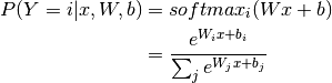
Mathematically, the probability that an input vector  is a member of a
class
is a member of a
class  , a value of a stochastic variable
  , can be written as:
The model’s prediction  is the class whose probability is maximal, specifically:

The code to do this in Theano is the following:
        # initialize with 0 the weights W as a matrix of shape (n_in, n_out)
        self.W = theano.shared(
            value=numpy.zeros(
                (n_in, n_out),
                dtype=theano.config.floatX
            ),
            name='W',
            borrow=True
        )
        # initialize the biases b as a vector of n_out 0s
        self.b = theano.shared(
            value=numpy.zeros(
                (n_out,),
                dtype=theano.config.floatX
            ),
            name='b',
            borrow=True
        )

        # symbolic expression for computing the matrix of class-membership
        # probabilities
        # Where:
        # W is a matrix where column-k represent the separation hyperplane for
        # class-k
        # x is a matrix where row-j  represents input training sample-j
        # b is a vector where element-k represent the free parameter of
        # hyperplane-k
        self.p_y_given_x = T.nnet.softmax(T.dot(input, self.W) + self.b)

        # symbolic description of how to compute prediction as class whose
        # probability is maximal
        self.y_pred = T.argmax(self.p_y_given_x, axis=1)
Since the parameters of the model must maintain a persistent state throughout
training, we allocate shared variables for  . This declares them both
as being symbolic Theano variables, but also initializes their contents. The
dot and softmax operators are then used to compute the vector
. This declares them both
as being symbolic Theano variables, but also initializes their contents. The
dot and softmax operators are then used to compute the vector  . The result
 p_y_given_x is a symbolic variable of vector-type.
To get the actual model prediction, we can use the T.argmax operator, which
will return the index at which p_y_given_x is maximal (i.e. the class with
maximum probability).
Now of course, the model we have defined so far does not do anything useful yet, since its parameters are still in their initial state. The following section will thus cover how to learn the optimal parameters.
Note
For a complete list of Theano ops, see: list of ops
Defining a Loss Function
Learning optimal model parameters involves minimizing a loss function. In the
case of multi-class logistic regression, it is very common to use the negative
log-likelihood as the loss. This is equivalent to maximizing the likelihood of the
data set  under the model parameterized by
  . Let
us first start by defining the likelihood
. Let
us first start by defining the likelihood  and loss
 :
:

While entire books are dedicated to the topic of minimization, gradient descent is by far the simplest method for minimizing arbitrary non-linear functions. This tutorial will use the method of stochastic gradient method with mini-batches (MSGD). See Stochastic Gradient Descent for more details.
The following Theano code defines the (symbolic) loss for a given minibatch:
        # y.shape[0] is (symbolically) the number of rows in y, i.e.,
        # number of examples (call it n) in the minibatch
        # T.arange(y.shape[0]) is a symbolic vector which will contain
        # [0,1,2,... n-1] T.log(self.p_y_given_x) is a matrix of
        # Log-Probabilities (call it LP) with one row per example and
        # one column per class LP[T.arange(y.shape[0]),y] is a vector
        # v containing [LP[0,y[0]], LP[1,y[1]], LP[2,y[2]], ...,
        # LP[n-1,y[n-1]]] and T.mean(LP[T.arange(y.shape[0]),y]) is
        # the mean (across minibatch examples) of the elements in v,
        # i.e., the mean log-likelihood across the minibatch.
        return -T.mean(T.log(self.p_y_given_x)[T.arange(y.shape[0]), y])
Note
Even though the loss is formally defined as the sum, over the data set,
of individual error terms, in practice, we use the mean (T.mean)
in the code. This allows for the learning rate choice to be less dependent
of the minibatch size.
Creating a LogisticRegression class
We now have all the tools we need to define a LogisticRegression class, which
encapsulates the basic behaviour of logistic regression. The code is very
similar to what we have covered so far, and should be self explanatory.
class LogisticRegression(object):
    """Multi-class Logistic Regression Class

    The logistic regression is fully described by a weight matrix :math:`W`
    and bias vector :math:`b`. Classification is done by projecting data
    points onto a set of hyperplanes, the distance to which is used to
    determine a class membership probability.
    """

    def __init__(self, input, n_in, n_out):
        """ Initialize the parameters of the logistic regression

        :type input: theano.tensor.TensorType
        :param input: symbolic variable that describes the input of the
                      architecture (one minibatch)

        :type n_in: int
        :param n_in: number of input units, the dimension of the space in
                     which the datapoints lie

        :type n_out: int
        :param n_out: number of output units, the dimension of the space in
                      which the labels lie

        """
        # start-snippet-1
        # initialize with 0 the weights W as a matrix of shape (n_in, n_out)
        self.W = theano.shared(
            value=numpy.zeros(
                (n_in, n_out),
                dtype=theano.config.floatX
            ),
            name='W',
            borrow=True
        )
        # initialize the biases b as a vector of n_out 0s
        self.b = theano.shared(
            value=numpy.zeros(
                (n_out,),
                dtype=theano.config.floatX
            ),
            name='b',
            borrow=True
        )

        # symbolic expression for computing the matrix of class-membership
        # probabilities
        # Where:
        # W is a matrix where column-k represent the separation hyperplane for
        # class-k
        # x is a matrix where row-j  represents input training sample-j
        # b is a vector where element-k represent the free parameter of
        # hyperplane-k
        self.p_y_given_x = T.nnet.softmax(T.dot(input, self.W) + self.b)

        # symbolic description of how to compute prediction as class whose
        # probability is maximal
        self.y_pred = T.argmax(self.p_y_given_x, axis=1)
        # end-snippet-1

        # parameters of the model
        self.params = [self.W, self.b]

        # keep track of model input
        self.input = input

    def negative_log_likelihood(self, y):
        """Return the mean of the negative log-likelihood of the prediction
        of this model under a given target distribution.

        .. math::

            \frac{1}{|\mathcal{D}|} \mathcal{L} (\theta=\{W,b\}, \mathcal{D}) =
            \frac{1}{|\mathcal{D}|} \sum_{i=0}^{|\mathcal{D}|}
                \log(P(Y=y^{(i)}|x^{(i)}, W,b)) \\
            \ell (\theta=\{W,b\}, \mathcal{D})

        :type y: theano.tensor.TensorType
        :param y: corresponds to a vector that gives for each example the
                  correct label

        Note: we use the mean instead of the sum so that
              the learning rate is less dependent on the batch size
        """
        # start-snippet-2
        # y.shape[0] is (symbolically) the number of rows in y, i.e.,
        # number of examples (call it n) in the minibatch
        # T.arange(y.shape[0]) is a symbolic vector which will contain
        # [0,1,2,... n-1] T.log(self.p_y_given_x) is a matrix of
        # Log-Probabilities (call it LP) with one row per example and
        # one column per class LP[T.arange(y.shape[0]),y] is a vector
        # v containing [LP[0,y[0]], LP[1,y[1]], LP[2,y[2]], ...,
        # LP[n-1,y[n-1]]] and T.mean(LP[T.arange(y.shape[0]),y]) is
        # the mean (across minibatch examples) of the elements in v,
        # i.e., the mean log-likelihood across the minibatch.
        return -T.mean(T.log(self.p_y_given_x)[T.arange(y.shape[0]), y])
        # end-snippet-2

    def errors(self, y):
        """Return a float representing the number of errors in the minibatch
        over the total number of examples of the minibatch ; zero one
        loss over the size of the minibatch

        :type y: theano.tensor.TensorType
        :param y: corresponds to a vector that gives for each example the
                  correct label
        """

        # check if y has same dimension of y_pred
        if y.ndim != self.y_pred.ndim:
            raise TypeError(
                'y should have the same shape as self.y_pred',
                ('y', y.type, 'y_pred', self.y_pred.type)
            )
        # check if y is of the correct datatype
        if y.dtype.startswith('int'):
            # the T.neq operator returns a vector of 0s and 1s, where 1
            # represents a mistake in prediction
            return T.mean(T.neq(self.y_pred, y))
        else:
            raise NotImplementedError()
We instantiate this class as follows:
    # generate symbolic variables for input (x and y represent a
    # minibatch)
    x = T.matrix('x')  # data, presented as rasterized images
    y = T.ivector('y')  # labels, presented as 1D vector of [int] labels

    # construct the logistic regression class
    # Each MNIST image has size 28*28
    classifier = LogisticRegression(input=x, n_in=28 * 28, n_out=10)
We start by allocating symbolic variables for the training inputs and
their corresponding classes  . Note that
 x and y are defined
outside the scope of the LogisticRegression object. Since the class
requires the input to build its graph, it is passed as a parameter of the
__init__ function. This is useful in case you want to connect instances of
such classes to form a deep network. The output of one layer can be passed as
the input of the layer above. (This tutorial does not build a multi-layer
network, but this code will be reused in future tutorials that do.)
Finally, we define a (symbolic) cost variable to minimize, using the instance
method classifier.negative_log_likelihood.
    # the cost we minimize during training is the negative log likelihood of
    # the model in symbolic format
    cost = classifier.negative_log_likelihood(y)
Note that x is an implicit symbolic input to the definition of cost,
because the symbolic variables of classifier were defined in terms of x
at initialization.
Learning the Model
To implement MSGD in most programming languages (C/C++, Matlab, Python), one
would start by manually deriving the expressions for the gradient of the loss
with respect to the parameters: in this case  ,
and
,
and  , This can get pretty tricky for complex
models, as expressions for
, This can get pretty tricky for complex
models, as expressions for  can get
fairly complex, especially when taking into account problems of numerical
stability.
can get
fairly complex, especially when taking into account problems of numerical
stability.
With Theano, this work is greatly simplified. It performs automatic differentiation and applies certain math transforms to improve numerical stability.
To get the gradients and
in Theano, simply do the following:
    g_W = T.grad(cost=cost, wrt=classifier.W)
    g_b = T.grad(cost=cost, wrt=classifier.b)
g_W and g_b are symbolic variables, which can be used as part
of a computation graph. The function train_model, which performs one step
of gradient descent, can then be defined as follows:
    # specify how to update the parameters of the model as a list of
    # (variable, update expression) pairs.
    updates = [(classifier.W, classifier.W - learning_rate * g_W),
               (classifier.b, classifier.b - learning_rate * g_b)]

    # compiling a Theano function `train_model` that returns the cost, but in
    # the same time updates the parameter of the model based on the rules
    # defined in `updates`
    train_model = theano.function(
        inputs=[index],
        outputs=cost,
        updates=updates,
        givens={
            x: train_set_x[index * batch_size: (index + 1) * batch_size],
            y: train_set_y[index * batch_size: (index + 1) * batch_size]
        }
    )
updates is a list of pairs. In each pair, the first element is the symbolic
variable to be updated in the step, and the second element is the symbolic
function for calculating its new value. Similarly, givens is a dictionary
whose keys are symbolic variables and whose values specify
their replacements during the step. The function train_model is then defined such
that:
- the input is the mini-batch index
indexthat, together with the batch size (which is not an input since it is fixed) defines with
corresponding labels - the return value is the cost/loss associated with the x, y defined by
the
index - on every function call, it will first replace
xandywith the slices from the training set specified byindex. Then, it will evaluate the cost associated with that minibatch and apply the operations defined by theupdateslist.
Each time train_model(index) is called, it will thus compute and return the
cost of a minibatch, while also performing a step of MSGD. The entire learning
algorithm thus consists in looping over all examples in the dataset, considering
all the examples in one minibatch at a time,
and repeatedly calling the train_model function.
Testing the model
As explained in Learning a Classifier, when testing the model we are
interested in the number of misclassified examples (and not only in the likelihood).
The LogisticRegression class therefore has an extra instance method, which
builds the symbolic graph for retrieving the number of misclassified examples in
each minibatch.
The code is as follows:
    def errors(self, y):
        """Return a float representing the number of errors in the minibatch
        over the total number of examples of the minibatch ; zero one
        loss over the size of the minibatch

        :type y: theano.tensor.TensorType
        :param y: corresponds to a vector that gives for each example the
                  correct label
        """

        # check if y has same dimension of y_pred
        if y.ndim != self.y_pred.ndim:
            raise TypeError(
                'y should have the same shape as self.y_pred',
                ('y', y.type, 'y_pred', self.y_pred.type)
            )
        # check if y is of the correct datatype
        if y.dtype.startswith('int'):
            # the T.neq operator returns a vector of 0s and 1s, where 1
            # represents a mistake in prediction
            return T.mean(T.neq(self.y_pred, y))
        else:
            raise NotImplementedError()
We then create a function test_model and a function validate_model,
which we can call to retrieve this value. As you will see shortly,
validate_model is key to our early-stopping implementation (see
Early-Stopping). These functions take a minibatch index and compute,
for the examples in that minibatch, the number that were misclassified by the
model. The only difference between them is that test_model draws its
minibatches from the testing set, while validate_model draws its from the
validation set.
    # compiling a Theano function that computes the mistakes that are made by
    # the model on a minibatch
    test_model = theano.function(
        inputs=[index],
        outputs=classifier.errors(y),
        givens={
            x: test_set_x[index * batch_size: (index + 1) * batch_size],
            y: test_set_y[index * batch_size: (index + 1) * batch_size]
        }
    )

    validate_model = theano.function(
        inputs=[index],
        outputs=classifier.errors(y),
        givens={
            x: valid_set_x[index * batch_size: (index + 1) * batch_size],
            y: valid_set_y[index * batch_size: (index + 1) * batch_size]
        }
    )
Putting it All Together
The finished product is as follows.
"""
This tutorial introduces logistic regression using Theano and stochastic
gradient descent.

Logistic regression is a probabilistic, linear classifier. It is parametrized
by a weight matrix :math:`W` and a bias vector :math:`b`. Classification is
done by projecting data points onto a set of hyperplanes, the distance to
which is used to determine a class membership probability.

Mathematically, this can be written as:

.. math::
  P(Y=i|x, W,b) &= softmax_i(W x + b) \\
                &= \frac {e^{W_i x + b_i}} {\sum_j e^{W_j x + b_j}}


The output of the model or prediction is then done by taking the argmax of
the vector whose i'th element is P(Y=i|x).

.. math::

  y_{pred} = argmax_i P(Y=i|x,W,b)


This tutorial presents a stochastic gradient descent optimization method
suitable for large datasets.


References:

    - textbooks: "Pattern Recognition and Machine Learning" -
                 Christopher M. Bishop, section 4.3.2

"""

from __future__ import print_function

__docformat__ = 'restructedtext en'

import six.moves.cPickle as pickle
import gzip
import os
import sys
import timeit

import numpy

import theano
import theano.tensor as T


class LogisticRegression(object):
    """Multi-class Logistic Regression Class

    The logistic regression is fully described by a weight matrix :math:`W`
    and bias vector :math:`b`. Classification is done by projecting data
    points onto a set of hyperplanes, the distance to which is used to
    determine a class membership probability.
    """

    def __init__(self, input, n_in, n_out):
        """ Initialize the parameters of the logistic regression

        :type input: theano.tensor.TensorType
        :param input: symbolic variable that describes the input of the
                      architecture (one minibatch)

        :type n_in: int
        :param n_in: number of input units, the dimension of the space in
                     which the datapoints lie

        :type n_out: int
        :param n_out: number of output units, the dimension of the space in
                      which the labels lie

        """
        # start-snippet-1
        # initialize with 0 the weights W as a matrix of shape (n_in, n_out)
        self.W = theano.shared(
            value=numpy.zeros(
                (n_in, n_out),
                dtype=theano.config.floatX
            ),
            name='W',
            borrow=True
        )
        # initialize the biases b as a vector of n_out 0s
        self.b = theano.shared(
            value=numpy.zeros(
                (n_out,),
                dtype=theano.config.floatX
            ),
            name='b',
            borrow=True
        )

        # symbolic expression for computing the matrix of class-membership
        # probabilities
        # Where:
        # W is a matrix where column-k represent the separation hyperplane for
        # class-k
        # x is a matrix where row-j  represents input training sample-j
        # b is a vector where element-k represent the free parameter of
        # hyperplane-k
        self.p_y_given_x = T.nnet.softmax(T.dot(input, self.W) + self.b)

        # symbolic description of how to compute prediction as class whose
        # probability is maximal
        self.y_pred = T.argmax(self.p_y_given_x, axis=1)
        # end-snippet-1

        # parameters of the model
        self.params = [self.W, self.b]

        # keep track of model input
        self.input = input

    def negative_log_likelihood(self, y):
        """Return the mean of the negative log-likelihood of the prediction
        of this model under a given target distribution.

        .. math::

            \frac{1}{|\mathcal{D}|} \mathcal{L} (\theta=\{W,b\}, \mathcal{D}) =
            \frac{1}{|\mathcal{D}|} \sum_{i=0}^{|\mathcal{D}|}
                \log(P(Y=y^{(i)}|x^{(i)}, W,b)) \\
            \ell (\theta=\{W,b\}, \mathcal{D})

        :type y: theano.tensor.TensorType
        :param y: corresponds to a vector that gives for each example the
                  correct label

        Note: we use the mean instead of the sum so that
              the learning rate is less dependent on the batch size
        """
        # start-snippet-2
        # y.shape[0] is (symbolically) the number of rows in y, i.e.,
        # number of examples (call it n) in the minibatch
        # T.arange(y.shape[0]) is a symbolic vector which will contain
        # [0,1,2,... n-1] T.log(self.p_y_given_x) is a matrix of
        # Log-Probabilities (call it LP) with one row per example and
        # one column per class LP[T.arange(y.shape[0]),y] is a vector
        # v containing [LP[0,y[0]], LP[1,y[1]], LP[2,y[2]], ...,
        # LP[n-1,y[n-1]]] and T.mean(LP[T.arange(y.shape[0]),y]) is
        # the mean (across minibatch examples) of the elements in v,
        # i.e., the mean log-likelihood across the minibatch.
        return -T.mean(T.log(self.p_y_given_x)[T.arange(y.shape[0]), y])
        # end-snippet-2

    def errors(self, y):
        """Return a float representing the number of errors in the minibatch
        over the total number of examples of the minibatch ; zero one
        loss over the size of the minibatch

        :type y: theano.tensor.TensorType
        :param y: corresponds to a vector that gives for each example the
                  correct label
        """

        # check if y has same dimension of y_pred
        if y.ndim != self.y_pred.ndim:
            raise TypeError(
                'y should have the same shape as self.y_pred',
                ('y', y.type, 'y_pred', self.y_pred.type)
            )
        # check if y is of the correct datatype
        if y.dtype.startswith('int'):
            # the T.neq operator returns a vector of 0s and 1s, where 1
            # represents a mistake in prediction
            return T.mean(T.neq(self.y_pred, y))
        else:
            raise NotImplementedError()


def load_data(dataset):
    ''' Loads the dataset

    :type dataset: string
    :param dataset: the path to the dataset (here MNIST)
    '''

    #############
    # LOAD DATA #
    #############

    # Download the MNIST dataset if it is not present
    data_dir, data_file = os.path.split(dataset)
    if data_dir == "" and not os.path.isfile(dataset):
        # Check if dataset is in the data directory.
        new_path = os.path.join(
            os.path.split(__file__)[0],
            "..",
            "data",
            dataset
        )
        if os.path.isfile(new_path) or data_file == 'mnist.pkl.gz':
            dataset = new_path

    if (not os.path.isfile(dataset)) and data_file == 'mnist.pkl.gz':
        from six.moves import urllib
        origin = (
            'http://www.iro.umontreal.ca/~lisa/deep/data/mnist/mnist.pkl.gz'
        )
        print('Downloading data from %s' % origin)
        urllib.request.urlretrieve(origin, dataset)

    print('... loading data')

    # Load the dataset
    with gzip.open(dataset, 'rb') as f:
        try:
            train_set, valid_set, test_set = pickle.load(f, encoding='latin1')
        except:
            train_set, valid_set, test_set = pickle.load(f)
    # train_set, valid_set, test_set format: tuple(input, target)
    # input is a numpy.ndarray of 2 dimensions (a matrix)
    # where each row corresponds to an example. target is a
    # numpy.ndarray of 1 dimension (vector) that has the same length as
    # the number of rows in the input. It should give the target
    # to the example with the same index in the input.

    def shared_dataset(data_xy, borrow=True):
        """ Function that loads the dataset into shared variables

        The reason we store our dataset in shared variables is to allow
        Theano to copy it into the GPU memory (when code is run on GPU).
        Since copying data into the GPU is slow, copying a minibatch everytime
        is needed (the default behaviour if the data is not in a shared
        variable) would lead to a large decrease in performance.
        """
        data_x, data_y = data_xy
        shared_x = theano.shared(numpy.asarray(data_x,
                                               dtype=theano.config.floatX),
                                 borrow=borrow)
        shared_y = theano.shared(numpy.asarray(data_y,
                                               dtype=theano.config.floatX),
                                 borrow=borrow)
        # When storing data on the GPU it has to be stored as floats
        # therefore we will store the labels as ``floatX`` as well
        # (``shared_y`` does exactly that). But during our computations
        # we need them as ints (we use labels as index, and if they are
        # floats it doesn't make sense) therefore instead of returning
        # ``shared_y`` we will have to cast it to int. This little hack
        # lets ous get around this issue
        return shared_x, T.cast(shared_y, 'int32')

    test_set_x, test_set_y = shared_dataset(test_set)
    valid_set_x, valid_set_y = shared_dataset(valid_set)
    train_set_x, train_set_y = shared_dataset(train_set)

    rval = [(train_set_x, train_set_y), (valid_set_x, valid_set_y),
            (test_set_x, test_set_y)]
    return rval


def sgd_optimization_mnist(learning_rate=0.13, n_epochs=1000,
                           dataset='mnist.pkl.gz',
                           batch_size=600):
    """
    Demonstrate stochastic gradient descent optimization of a log-linear
    model

    This is demonstrated on MNIST.

    :type learning_rate: float
    :param learning_rate: learning rate used (factor for the stochastic
                          gradient)

    :type n_epochs: int
    :param n_epochs: maximal number of epochs to run the optimizer

    :type dataset: string
    :param dataset: the path of the MNIST dataset file from
                 http://www.iro.umontreal.ca/~lisa/deep/data/mnist/mnist.pkl.gz

    """
    datasets = load_data(dataset)

    train_set_x, train_set_y = datasets[0]
    valid_set_x, valid_set_y = datasets[1]
    test_set_x, test_set_y = datasets[2]

    # compute number of minibatches for training, validation and testing
    n_train_batches = train_set_x.get_value(borrow=True).shape[0] // batch_size
    n_valid_batches = valid_set_x.get_value(borrow=True).shape[0] // batch_size
    n_test_batches = test_set_x.get_value(borrow=True).shape[0] // batch_size

    ######################
    # BUILD ACTUAL MODEL #
    ######################
    print('... building the model')

    # allocate symbolic variables for the data
    index = T.lscalar()  # index to a [mini]batch

    # generate symbolic variables for input (x and y represent a
    # minibatch)
    x = T.matrix('x')  # data, presented as rasterized images
    y = T.ivector('y')  # labels, presented as 1D vector of [int] labels

    # construct the logistic regression class
    # Each MNIST image has size 28*28
    classifier = LogisticRegression(input=x, n_in=28 * 28, n_out=10)

    # the cost we minimize during training is the negative log likelihood of
    # the model in symbolic format
    cost = classifier.negative_log_likelihood(y)

    # compiling a Theano function that computes the mistakes that are made by
    # the model on a minibatch
    test_model = theano.function(
        inputs=[index],
        outputs=classifier.errors(y),
        givens={
            x: test_set_x[index * batch_size: (index + 1) * batch_size],
            y: test_set_y[index * batch_size: (index + 1) * batch_size]
        }
    )

    validate_model = theano.function(
        inputs=[index],
        outputs=classifier.errors(y),
        givens={
            x: valid_set_x[index * batch_size: (index + 1) * batch_size],
            y: valid_set_y[index * batch_size: (index + 1) * batch_size]
        }
    )

    # compute the gradient of cost with respect to theta = (W,b)
    g_W = T.grad(cost=cost, wrt=classifier.W)
    g_b = T.grad(cost=cost, wrt=classifier.b)

    # start-snippet-3
    # specify how to update the parameters of the model as a list of
    # (variable, update expression) pairs.
    updates = [(classifier.W, classifier.W - learning_rate * g_W),
               (classifier.b, classifier.b - learning_rate * g_b)]

    # compiling a Theano function `train_model` that returns the cost, but in
    # the same time updates the parameter of the model based on the rules
    # defined in `updates`
    train_model = theano.function(
        inputs=[index],
        outputs=cost,
        updates=updates,
        givens={
            x: train_set_x[index * batch_size: (index + 1) * batch_size],
            y: train_set_y[index * batch_size: (index + 1) * batch_size]
        }
    )
    # end-snippet-3

    ###############
    # TRAIN MODEL #
    ###############
    print('... training the model')
    # early-stopping parameters
    patience = 5000  # look as this many examples regardless
    patience_increase = 2  # wait this much longer when a new best is
                                  # found
    improvement_threshold = 0.995  # a relative improvement of this much is
                                  # considered significant
    validation_frequency = min(n_train_batches, patience // 2)
                                  # go through this many
                                  # minibatche before checking the network
                                  # on the validation set; in this case we
                                  # check every epoch

    best_validation_loss = numpy.inf
    test_score = 0.
    start_time = timeit.default_timer()

    done_looping = False
    epoch = 0
    while (epoch < n_epochs) and (not done_looping):
        epoch = epoch + 1
        for minibatch_index in range(n_train_batches):

            minibatch_avg_cost = train_model(minibatch_index)
            # iteration number
            iter = (epoch - 1) * n_train_batches + minibatch_index

            if (iter + 1) % validation_frequency == 0:
                # compute zero-one loss on validation set
                validation_losses = [validate_model(i)
                                     for i in range(n_valid_batches)]
                this_validation_loss = numpy.mean(validation_losses)

                print(
                    'epoch %i, minibatch %i/%i, validation error %f %%' %
                    (
                        epoch,
                        minibatch_index + 1,
                        n_train_batches,
                        this_validation_loss * 100.
                    )
                )

                # if we got the best validation score until now
                if this_validation_loss < best_validation_loss:
                    #improve patience if loss improvement is good enough
                    if this_validation_loss < best_validation_loss *  \
                       improvement_threshold:
                        patience = max(patience, iter * patience_increase)

                    best_validation_loss = this_validation_loss
                    # test it on the test set

                    test_losses = [test_model(i)
                                   for i in range(n_test_batches)]
                    test_score = numpy.mean(test_losses)

                    print(
                        (
                            '     epoch %i, minibatch %i/%i, test error of'
                            ' best model %f %%'
                        ) %
                        (
                            epoch,
                            minibatch_index + 1,
                            n_train_batches,
                            test_score * 100.
                        )
                    )

                    # save the best model
                    with open('best_model.pkl', 'wb') as f:
                        pickle.dump(classifier, f)

            if patience <= iter:
                done_looping = True
                break

    end_time = timeit.default_timer()
    print(
        (
            'Optimization complete with best validation score of %f %%,'
            'with test performance %f %%'
        )
        % (best_validation_loss * 100., test_score * 100.)
    )
    print('The code run for %d epochs, with %f epochs/sec' % (
        epoch, 1. * epoch / (end_time - start_time)))
    print(('The code for file ' +
           os.path.split(__file__)[1] +
           ' ran for %.1fs' % ((end_time - start_time))), file=sys.stderr)


def predict():
    """
    An example of how to load a trained model and use it
    to predict labels.
    """

    # load the saved model
    classifier = pickle.load(open('best_model.pkl'))

    # compile a predictor function
    predict_model = theano.function(
        inputs=[classifier.input],
        outputs=classifier.y_pred)

    # We can test it on some examples from test test
    dataset='mnist.pkl.gz'
    datasets = load_data(dataset)
    test_set_x, test_set_y = datasets[2]
    test_set_x = test_set_x.get_value()

    predicted_values = predict_model(test_set_x[:10])
    print("Predicted values for the first 10 examples in test set:")
    print(predicted_values)


if __name__ == '__main__':
    sgd_optimization_mnist()
The user can learn to classify MNIST digits with SGD logistic regression, by typing, from within the DeepLearningTutorials folder:
python code/logistic_sgd.py
The output one should expect is of the form:
...
epoch 72, minibatch 83/83, validation error 7.510417 %
     epoch 72, minibatch 83/83, test error of best model 7.510417 %
epoch 73, minibatch 83/83, validation error 7.500000 %
     epoch 73, minibatch 83/83, test error of best model 7.489583 %
Optimization complete with best validation score of 7.500000 %,with test performance 7.489583 %
The code run for 74 epochs, with 1.936983 epochs/sec
On an Intel(R) Core(TM)2 Duo CPU E8400 @ 3.00 Ghz the code runs with approximately 1.936 epochs/sec and it took 75 epochs to reach a test error of 7.489%. On the GPU the code does almost 10.0 epochs/sec. For this instance we used a batch size of 600.
Prediction Using a Trained Model
sgd_optimization_mnist serialize and pickle the model each time new
lowest validation error is reached. We can reload this model and predict
labels of new data. predict function shows an example of how
this could be done.
def predict():
    """
    An example of how to load a trained model and use it
    to predict labels.
    """

    # load the saved model
    classifier = pickle.load(open('best_model.pkl'))

    # compile a predictor function
    predict_model = theano.function(
        inputs=[classifier.input],
        outputs=classifier.y_pred)

    # We can test it on some examples from test test
    dataset='mnist.pkl.gz'
    datasets = load_data(dataset)
    test_set_x, test_set_y = datasets[2]
    test_set_x = test_set_x.get_value()

    predicted_values = predict_model(test_set_x[:10])
    print("Predicted values for the first 10 examples in test set:")
    print(predicted_values)
Footnotes
| [1] | For smaller datasets and simpler models, more sophisticated descent algorithms can be more effective. The sample code logistic_cg.py demonstrates how to use SciPy’s conjugate gradient solver with Theano on the logistic regression task. |