Denoising Autoencoders (dA)¶

Note

This section assumes the reader has already read through Classifying MNIST digits using Logistic Regression and Multilayer Perceptron. Additionally it uses the following Theano functions and concepts: T.tanh, shared variables, basic arithmetic ops, T.grad, Random numbers, floatX. If you intend to run the code on GPU also read GPU.

Note

The code for this section is available for download here.

The Denoising Autoencoder (dA) is an extension of a classical autoencoder and it was introduced as a building block for deep networks in [Vincent08]. We will start the tutorial with a short discussion on Autoencoders.

Autoencoders¶

See section 4.6 of [Bengio09] for an overview of auto-encoders. An autoencoder takes an input $\mathbf{x} \in [0,1]^d$ and first maps it (with an encoder) to a hidden representation $\mathbf{y} \in [0,1]^{d'}$ through a deterministic mapping, e.g.:

$\mathbf{y} = s(\mathbf{W}\mathbf{x} + \mathbf{b})$

Where $s$ is a non-linearity such as the sigmoid. The latent representation $\mathbf{y}$ , or code is then mapped back (with a decoder) into a reconstruction $\mathbf{z}$ of the same shape as $\mathbf{x}$ . The mapping happens through a similar transformation, e.g.:

$\mathbf{z} = s(\mathbf{W'}\mathbf{y} + \mathbf{b'})$

(Here, the prime symbol does not indicate matrix transposition.) $\mathbf{z}$ should be seen as a prediction of $\mathbf{x}$ , given the code $\mathbf{y}$ . Optionally, the weight matrix $\mathbf{W'}$ of the reverse mapping may be constrained to be the transpose of the forward mapping: $\mathbf{W'} = \mathbf{W}^T$ . This is referred to as tied weights. The parameters of this model (namely $\mathbf{W}$ , $\mathbf{b}$ , $\mathbf{b'}$ and, if one doesn’t use tied weights, also $\mathbf{W'}$ ) are optimized such that the average reconstruction error is minimized.

The reconstruction error can be measured in many ways, depending on the appropriate distributional assumptions on the input given the code. The traditional squared error $L(\mathbf{x} \mathbf{z}) = || \mathbf{x} - \mathbf{z} ||^2$ , can be used. If the input is interpreted as either bit vectors or vectors of bit probabilities, cross-entropy of the reconstruction can be used:

$L_{H} (\mathbf{x}, \mathbf{z}) = - \sum^d_{k=1}[\mathbf{x}_k \log \mathbf{z}_k + (1 - \mathbf{x}_k)\log(1 - \mathbf{z}_k)]$

The hope is that the code $\mathbf{y}$ is a distributed representation that captures the coordinates along the main factors of variation in the data. This is similar to the way the projection on principal components would capture the main factors of variation in the data. Indeed, if there is one linear hidden layer (the code) and the mean squared error criterion is used to train the network, then the $k$ hidden units learn to project the input in the span of the first $k$ principal components of the data. If the hidden layer is non-linear, the auto-encoder behaves differently from PCA, with the ability to capture multi-modal aspects of the input distribution. The departure from PCA becomes even more important when we consider stacking multiple encoders (and their corresponding decoders) when building a deep auto-encoder [Hinton06].

Because $\mathbf{y}$ is viewed as a lossy compression of $\mathbf{x}$ , it cannot be a good (small-loss) compression for all $\mathbf{x}$ . Optimization makes it a good compression for training examples, and hopefully for other inputs as well, but not for arbitrary inputs. That is the sense in which an auto-encoder generalizes: it gives low reconstruction error on test examples from the same distribution as the training examples, but generally high reconstruction error on samples randomly chosen from the input space.

We want to implement an auto-encoder using Theano, in the form of a class, that could be afterwards used in constructing a stacked autoencoder. The first step is to create shared variables for the parameters of the autoencoder $\mathbf{W}$ , $\mathbf{b}$ and $\mathbf{b'}$ . (Since we are using tied weights in this tutorial, $\mathbf{W}^T$ will be used for $\mathbf{W'}$ ):

    def __init__(
        self,
        numpy_rng,
        theano_rng=None,
        input=None,
        n_visible=784,
        n_hidden=500,
        W=None,
        bhid=None,
        bvis=None
    ):
        """
        Initialize the dA class by specifying the number of visible units (the
        dimension d of the input ), the number of hidden units ( the dimension
        d' of the latent or hidden space ) and the corruption level. The
        constructor also receives symbolic variables for the input, weights and
        bias. Such a symbolic variables are useful when, for example the input
        is the result of some computations, or when weights are shared between
        the dA and an MLP layer. When dealing with SdAs this always happens,
        the dA on layer 2 gets as input the output of the dA on layer 1,
        and the weights of the dA are used in the second stage of training
        to construct an MLP.

        :type numpy_rng: numpy.random.RandomState
        :param numpy_rng: number random generator used to generate weights

        :type theano_rng: theano.tensor.shared_randomstreams.RandomStreams
        :param theano_rng: Theano random generator; if None is given one is
                     generated based on a seed drawn from `rng`

        :type input: theano.tensor.TensorType
        :param input: a symbolic description of the input or None for
                      standalone dA

        :type n_visible: int
        :param n_visible: number of visible units

        :type n_hidden: int
        :param n_hidden:  number of hidden units

        :type W: theano.tensor.TensorType
        :param W: Theano variable pointing to a set of weights that should be
                  shared belong the dA and another architecture; if dA should
                  be standalone set this to None

        :type bhid: theano.tensor.TensorType
        :param bhid: Theano variable pointing to a set of biases values (for
                     hidden units) that should be shared belong dA and another
                     architecture; if dA should be standalone set this to None

        :type bvis: theano.tensor.TensorType
        :param bvis: Theano variable pointing to a set of biases values (for
                     visible units) that should be shared belong dA and another
                     architecture; if dA should be standalone set this to None


        """
        self.n_visible = n_visible
        self.n_hidden = n_hidden

        # create a Theano random generator that gives symbolic random values
        if not theano_rng:
            theano_rng = RandomStreams(numpy_rng.randint(2 ** 30))

        # note : W' was written as `W_prime` and b' as `b_prime`
        if not W:
            # W is initialized with `initial_W` which is uniformely sampled
            # from -4*sqrt(6./(n_visible+n_hidden)) and
            # 4*sqrt(6./(n_hidden+n_visible))the output of uniform if
            # converted using asarray to dtype
            # theano.config.floatX so that the code is runable on GPU
            initial_W = numpy.asarray(
                numpy_rng.uniform(
                    low=-4 * numpy.sqrt(6. / (n_hidden + n_visible)),
                    high=4 * numpy.sqrt(6. / (n_hidden + n_visible)),
                    size=(n_visible, n_hidden)
                ),
                dtype=theano.config.floatX
            )
            W = theano.shared(value=initial_W, name='W', borrow=True)

        if not bvis:
            bvis = theano.shared(
                value=numpy.zeros(
                    n_visible,
                    dtype=theano.config.floatX
                ),
                borrow=True
            )

        if not bhid:
            bhid = theano.shared(
                value=numpy.zeros(
                    n_hidden,
                    dtype=theano.config.floatX
                ),
                name='b',
                borrow=True
            )

        self.W = W
        # b corresponds to the bias of the hidden
        self.b = bhid
        # b_prime corresponds to the bias of the visible
        self.b_prime = bvis
        # tied weights, therefore W_prime is W transpose
        self.W_prime = self.W.T
        self.theano_rng = theano_rng
        # if no input is given, generate a variable representing the input
        if input is None:
            # we use a matrix because we expect a minibatch of several
            # examples, each example being a row
            self.x = T.dmatrix(name='input')
        else:
            self.x = input

        self.params = [self.W, self.b, self.b_prime]

Note that we pass the symbolic input to the autoencoder as a parameter. This is so that we can concatenate layers of autoencoders to form a deep network: the symbolic output (the $\mathbf{y}$ above) of layer $k$ will be the symbolic input of layer $k+1$ .

Now we can express the computation of the latent representation and of the reconstructed signal:

    def get_hidden_values(self, input):
        """ Computes the values of the hidden layer """
        return T.nnet.sigmoid(T.dot(input, self.W) + self.b)

    def get_reconstructed_input(self, hidden):
        """Computes the reconstructed input given the values of the
        hidden layer

        """
        return T.nnet.sigmoid(T.dot(hidden, self.W_prime) + self.b_prime)

And using these functions we can compute the cost and the updates of one stochastic gradient descent step:

    def get_cost_updates(self, corruption_level, learning_rate):
        """ This function computes the cost and the updates for one trainng
        step of the dA """

        tilde_x = self.get_corrupted_input(self.x, corruption_level)
        y = self.get_hidden_values(tilde_x)
        z = self.get_reconstructed_input(y)
        # note : we sum over the size of a datapoint; if we are using
        #        minibatches, L will be a vector, with one entry per
        #        example in minibatch
        L = - T.sum(self.x * T.log(z) + (1 - self.x) * T.log(1 - z), axis=1)
        # note : L is now a vector, where each element is the
        #        cross-entropy cost of the reconstruction of the
        #        corresponding example of the minibatch. We need to
        #        compute the average of all these to get the cost of
        #        the minibatch
        cost = T.mean(L)

        # compute the gradients of the cost of the `dA` with respect
        # to its parameters
        gparams = T.grad(cost, self.params)
        # generate the list of updates
        updates = [
            (param, param - learning_rate * gparam)
            for param, gparam in zip(self.params, gparams)
        ]

        return (cost, updates)

We can now define a function that applied iteratively will update the parameters W, b and b_prime such that the reconstruction cost is approximately minimized.

    da = dA(
        numpy_rng=rng,
        theano_rng=theano_rng,
        input=x,
        n_visible=28 * 28,
        n_hidden=500
    )

    cost, updates = da.get_cost_updates(
        corruption_level=0.,
        learning_rate=learning_rate
    )

    train_da = theano.function(
        [index],
        cost,
        updates=updates,
        givens={
            x: train_set_x[index * batch_size: (index + 1) * batch_size]
        }
    )

    start_time = timeit.default_timer()

    ############
    # TRAINING #
    ############

    # go through training epochs
    for epoch in range(training_epochs):
        # go through trainng set
        c = []
        for batch_index in range(n_train_batches):
            c.append(train_da(batch_index))

        print('Training epoch %d, cost ' % epoch, numpy.mean(c, dtype='float64'))

    end_time = timeit.default_timer()

    training_time = (end_time - start_time)

    print(('The no corruption code for file ' +
           os.path.split(__file__)[1] +
           ' ran for %.2fm' % ((training_time) / 60.)), file=sys.stderr)
    image = Image.fromarray(
        tile_raster_images(X=da.W.get_value(borrow=True).T,
                           img_shape=(28, 28), tile_shape=(10, 10),
                           tile_spacing=(1, 1)))
    image.save('filters_corruption_0.png')

    # start-snippet-3
    #####################################
    # BUILDING THE MODEL CORRUPTION 30% #
    #####################################

    rng = numpy.random.RandomState(123)
    theano_rng = RandomStreams(rng.randint(2 ** 30))

    da = dA(
        numpy_rng=rng,
        theano_rng=theano_rng,
        input=x,
        n_visible=28 * 28,
        n_hidden=500
    )

    cost, updates = da.get_cost_updates(
        corruption_level=0.3,
        learning_rate=learning_rate
    )

    train_da = theano.function(
        [index],
        cost,
        updates=updates,
        givens={
            x: train_set_x[index * batch_size: (index + 1) * batch_size]
        }
    )

    start_time = timeit.default_timer()

    ############
    # TRAINING #
    ############

    # go through training epochs
    for epoch in range(training_epochs):
        # go through trainng set
        c = []
        for batch_index in range(n_train_batches):
            c.append(train_da(batch_index))

        print('Training epoch %d, cost ' % epoch, numpy.mean(c, dtype='float64'))

    end_time = timeit.default_timer()

    training_time = (end_time - start_time)

    print(('The 30% corruption code for file ' +
           os.path.split(__file__)[1] +
           ' ran for %.2fm' % (training_time / 60.)), file=sys.stderr)
    # end-snippet-3

    # start-snippet-4
    image = Image.fromarray(tile_raster_images(
        X=da.W.get_value(borrow=True).T,
        img_shape=(28, 28), tile_shape=(10, 10),
        tile_spacing=(1, 1)))
    image.save('filters_corruption_30.png')
    # end-snippet-4

    os.chdir('../')


if __name__ == '__main__':
    test_dA()

If there is no constraint besides minimizing the reconstruction error, one might expect an auto-encoder with $n$ inputs and an encoding of dimension $n$ (or greater) to learn the identity function, merely mapping an input to its copy. Such an autoencoder would not differentiate test examples (from the training distribution) from other input configurations.

Surprisingly, experiments reported in [Bengio07] suggest that, in practice, when trained with stochastic gradient descent, non-linear auto-encoders with more hidden units than inputs (called overcomplete) yield useful representations. (Here, “useful” means that a network taking the encoding as input has low classification error.)

A simple explanation is that stochastic gradient descent with early stopping is similar to an L2 regularization of the parameters. To achieve perfect reconstruction of continuous inputs, a one-hidden layer auto-encoder with non-linear hidden units (exactly like in the above code) needs very small weights in the first (encoding) layer, to bring the non-linearity of the hidden units into their linear regime, and very large weights in the second (decoding) layer. With binary inputs, very large weights are also needed to completely minimize the reconstruction error. Since the implicit or explicit regularization makes it difficult to reach large-weight solutions, the optimization algorithm finds encodings which only work well for examples similar to those in the training set, which is what we want. It means that the representation is exploiting statistical regularities present in the training set, rather than merely learning to replicate the input.

There are other ways by which an auto-encoder with more hidden units than inputs could be prevented from learning the identity function, capturing something useful about the input in its hidden representation. One is the addition of sparsity (forcing many of the hidden units to be zero or near-zero). Sparsity has been exploited very successfully by many [Ranzato07] [Lee08]. Another is to add randomness in the transformation from input to reconstruction. This technique is used in Restricted Boltzmann Machines (discussed later in Restricted Boltzmann Machines (RBM)), as well as in Denoising Auto-Encoders, discussed below.

Denoising Autoencoders¶

The idea behind denoising autoencoders is simple. In order to force the hidden layer to discover more robust features and prevent it from simply learning the identity, we train the autoencoder to reconstruct the input from a corrupted version of it.

The denoising auto-encoder is a stochastic version of the auto-encoder. Intuitively, a denoising auto-encoder does two things: try to encode the input (preserve the information about the input), and try to undo the effect of a corruption process stochastically applied to the input of the auto-encoder. The latter can only be done by capturing the statistical dependencies between the inputs. The denoising auto-encoder can be understood from different perspectives (the manifold learning perspective, stochastic operator perspective, bottom-up – information theoretic perspective, top-down – generative model perspective), all of which are explained in [Vincent08]. See also section 7.2 of [Bengio09] for an overview of auto-encoders.

In [Vincent08], the stochastic corruption process randomly sets some of the inputs (as many as half of them) to zero. Hence the denoising auto-encoder is trying to predict the corrupted (i.e. missing) values from the uncorrupted (i.e., non-missing) values, for randomly selected subsets of missing patterns. Note how being able to predict any subset of variables from the rest is a sufficient condition for completely capturing the joint distribution between a set of variables (this is how Gibbs sampling works).

To convert the autoencoder class into a denoising autoencoder class, all we need to do is to add a stochastic corruption step operating on the input. The input can be corrupted in many ways, but in this tutorial we will stick to the original corruption mechanism of randomly masking entries of the input by making them zero. The code below does just that:

    def get_corrupted_input(self, input, corruption_level):
        """This function keeps ``1-corruption_level`` entries of the inputs the
        same and zero-out randomly selected subset of size ``corruption_level``
        Note : first argument of theano.rng.binomial is the shape(size) of
               random numbers that it should produce
               second argument is the number of trials
               third argument is the probability of success of any trial

                this will produce an array of 0s and 1s where 1 has a
                probability of 1 - ``corruption_level`` and 0 with
                ``corruption_level``

                The binomial function return int64 data type by
                default.  int64 multiplicated by the input
                type(floatX) always return float64.  To keep all data
                in floatX when floatX is float32, we set the dtype of
                the binomial to floatX. As in our case the value of
                the binomial is always 0 or 1, this don't change the
                result. This is needed to allow the gpu to work
                correctly as it only support float32 for now.

        """
        return self.theano_rng.binomial(size=input.shape, n=1,
                                        p=1 - corruption_level,
                                        dtype=theano.config.floatX) * input

In the stacked autoencoder class (Stacked Autoencoders) the weights of the dA class have to be shared with those of a corresponding sigmoid layer. For this reason, the constructor of the dA also gets Theano variables pointing to the shared parameters. If those parameters are left to None, new ones will be constructed.

The final denoising autoencoder class becomes:

class dA(object):
    """Denoising Auto-Encoder class (dA)

    A denoising autoencoders tries to reconstruct the input from a corrupted
    version of it by projecting it first in a latent space and reprojecting
    it afterwards back in the input space. Please refer to Vincent et al.,2008
    for more details. If x is the input then equation (1) computes a partially
    destroyed version of x by means of a stochastic mapping q_D. Equation (2)
    computes the projection of the input into the latent space. Equation (3)
    computes the reconstruction of the input, while equation (4) computes the
    reconstruction error.

    .. math::

        \tilde{x} ~ q_D(\tilde{x}|x)                                     (1)

        y = s(W \tilde{x} + b)                                           (2)

        x = s(W' y  + b')                                                (3)

        L(x,z) = -sum_{k=1}^d [x_k \log z_k + (1-x_k) \log( 1-z_k)]      (4)

    """

    def __init__(
        self,
        numpy_rng,
        theano_rng=None,
        input=None,
        n_visible=784,
        n_hidden=500,
        W=None,
        bhid=None,
        bvis=None
    ):
        """
        Initialize the dA class by specifying the number of visible units (the
        dimension d of the input ), the number of hidden units ( the dimension
        d' of the latent or hidden space ) and the corruption level. The
        constructor also receives symbolic variables for the input, weights and
        bias. Such a symbolic variables are useful when, for example the input
        is the result of some computations, or when weights are shared between
        the dA and an MLP layer. When dealing with SdAs this always happens,
        the dA on layer 2 gets as input the output of the dA on layer 1,
        and the weights of the dA are used in the second stage of training
        to construct an MLP.

        :type numpy_rng: numpy.random.RandomState
        :param numpy_rng: number random generator used to generate weights

        :type theano_rng: theano.tensor.shared_randomstreams.RandomStreams
        :param theano_rng: Theano random generator; if None is given one is
                     generated based on a seed drawn from `rng`

        :type input: theano.tensor.TensorType
        :param input: a symbolic description of the input or None for
                      standalone dA

        :type n_visible: int
        :param n_visible: number of visible units

        :type n_hidden: int
        :param n_hidden:  number of hidden units

        :type W: theano.tensor.TensorType
        :param W: Theano variable pointing to a set of weights that should be
                  shared belong the dA and another architecture; if dA should
                  be standalone set this to None

        :type bhid: theano.tensor.TensorType
        :param bhid: Theano variable pointing to a set of biases values (for
                     hidden units) that should be shared belong dA and another
                     architecture; if dA should be standalone set this to None

        :type bvis: theano.tensor.TensorType
        :param bvis: Theano variable pointing to a set of biases values (for
                     visible units) that should be shared belong dA and another
                     architecture; if dA should be standalone set this to None


        """
        self.n_visible = n_visible
        self.n_hidden = n_hidden

        # create a Theano random generator that gives symbolic random values
        if not theano_rng:
            theano_rng = RandomStreams(numpy_rng.randint(2 ** 30))

        # note : W' was written as `W_prime` and b' as `b_prime`
        if not W:
            # W is initialized with `initial_W` which is uniformely sampled
            # from -4*sqrt(6./(n_visible+n_hidden)) and
            # 4*sqrt(6./(n_hidden+n_visible))the output of uniform if
            # converted using asarray to dtype
            # theano.config.floatX so that the code is runable on GPU
            initial_W = numpy.asarray(
                numpy_rng.uniform(
                    low=-4 * numpy.sqrt(6. / (n_hidden + n_visible)),
                    high=4 * numpy.sqrt(6. / (n_hidden + n_visible)),
                    size=(n_visible, n_hidden)
                ),
                dtype=theano.config.floatX
            )
            W = theano.shared(value=initial_W, name='W', borrow=True)

        if not bvis:
            bvis = theano.shared(
                value=numpy.zeros(
                    n_visible,
                    dtype=theano.config.floatX
                ),
                borrow=True
            )

        if not bhid:
            bhid = theano.shared(
                value=numpy.zeros(
                    n_hidden,
                    dtype=theano.config.floatX
                ),
                name='b',
                borrow=True
            )

        self.W = W
        # b corresponds to the bias of the hidden
        self.b = bhid
        # b_prime corresponds to the bias of the visible
        self.b_prime = bvis
        # tied weights, therefore W_prime is W transpose
        self.W_prime = self.W.T
        self.theano_rng = theano_rng
        # if no input is given, generate a variable representing the input
        if input is None:
            # we use a matrix because we expect a minibatch of several
            # examples, each example being a row
            self.x = T.dmatrix(name='input')
        else:
            self.x = input

        self.params = [self.W, self.b, self.b_prime]

    def get_corrupted_input(self, input, corruption_level):
        """This function keeps ``1-corruption_level`` entries of the inputs the
        same and zero-out randomly selected subset of size ``corruption_level``
        Note : first argument of theano.rng.binomial is the shape(size) of
               random numbers that it should produce
               second argument is the number of trials
               third argument is the probability of success of any trial

                this will produce an array of 0s and 1s where 1 has a
                probability of 1 - ``corruption_level`` and 0 with
                ``corruption_level``

                The binomial function return int64 data type by
                default.  int64 multiplicated by the input
                type(floatX) always return float64.  To keep all data
                in floatX when floatX is float32, we set the dtype of
                the binomial to floatX. As in our case the value of
                the binomial is always 0 or 1, this don't change the
                result. This is needed to allow the gpu to work
                correctly as it only support float32 for now.

        """
        return self.theano_rng.binomial(size=input.shape, n=1,
                                        p=1 - corruption_level,
                                        dtype=theano.config.floatX) * input

    def get_hidden_values(self, input):
        """ Computes the values of the hidden layer """
        return T.nnet.sigmoid(T.dot(input, self.W) + self.b)

    def get_reconstructed_input(self, hidden):
        """Computes the reconstructed input given the values of the
        hidden layer

        """
        return T.nnet.sigmoid(T.dot(hidden, self.W_prime) + self.b_prime)

    def get_cost_updates(self, corruption_level, learning_rate):
        """ This function computes the cost and the updates for one trainng
        step of the dA """

        tilde_x = self.get_corrupted_input(self.x, corruption_level)
        y = self.get_hidden_values(tilde_x)
        z = self.get_reconstructed_input(y)
        # note : we sum over the size of a datapoint; if we are using
        #        minibatches, L will be a vector, with one entry per
        #        example in minibatch
        L = - T.sum(self.x * T.log(z) + (1 - self.x) * T.log(1 - z), axis=1)
        # note : L is now a vector, where each element is the
        #        cross-entropy cost of the reconstruction of the
        #        corresponding example of the minibatch. We need to
        #        compute the average of all these to get the cost of
        #        the minibatch
        cost = T.mean(L)

        # compute the gradients of the cost of the `dA` with respect
        # to its parameters
        gparams = T.grad(cost, self.params)
        # generate the list of updates
        updates = [
            (param, param - learning_rate * gparam)
            for param, gparam in zip(self.params, gparams)
        ]

        return (cost, updates)

Putting it All Together¶

It is easy now to construct an instance of our dA class and train it.

    # allocate symbolic variables for the data
    index = T.lscalar()    # index to a [mini]batch
    x = T.matrix('x')  # the data is presented as rasterized images

    #####################################
    # BUILDING THE MODEL CORRUPTION 30% #
    #####################################

    rng = numpy.random.RandomState(123)
    theano_rng = RandomStreams(rng.randint(2 ** 30))

    da = dA(
        numpy_rng=rng,
        theano_rng=theano_rng,
        input=x,
        n_visible=28 * 28,
        n_hidden=500
    )

    cost, updates = da.get_cost_updates(
        corruption_level=0.3,
        learning_rate=learning_rate
    )

    train_da = theano.function(
        [index],
        cost,
        updates=updates,
        givens={
            x: train_set_x[index * batch_size: (index + 1) * batch_size]
        }
    )

    start_time = timeit.default_timer()

    ############
    # TRAINING #
    ############

    # go through training epochs
    for epoch in range(training_epochs):
        # go through trainng set
        c = []
        for batch_index in range(n_train_batches):
            c.append(train_da(batch_index))

        print('Training epoch %d, cost ' % epoch, numpy.mean(c, dtype='float64'))

    end_time = timeit.default_timer()

    training_time = (end_time - start_time)

    print(('The 30% corruption code for file ' +
           os.path.split(__file__)[1] +
           ' ran for %.2fm' % (training_time / 60.)), file=sys.stderr)

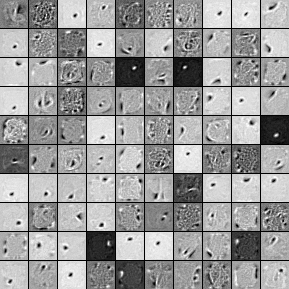
In order to get a feeling of what the network learned we are going to plot the filters (defined by the weight matrix). Bear in mind, however, that this does not provide the entire story, since we neglect the biases and plot the weights up to a multiplicative constant (weights are converted to values between 0 and 1).

To plot our filters we will need the help of tile_raster_images (see Plotting Samples and Filters) so we urge the reader to study it. Also using the help of the Python Image Library, the following lines of code will save the filters as an image:

    image = Image.fromarray(tile_raster_images(
        X=da.W.get_value(borrow=True).T,
        img_shape=(28, 28), tile_shape=(10, 10),
        tile_spacing=(1, 1)))
    image.save('filters_corruption_30.png')

Running the Code¶

To run the code:

python dA.py

The resulted filters when we do not use any noise are:

The filters for 30 percent noise:

Table Of Contents

Previous topic

Next topic

This Page